Logistic Regression_3

Question

For this exercise, you will use logistic regression and neural networks to recognize handwritten digits (from 0 to 9). Automated handwritten digit recognition is widely used today - from recognizing zip codes (postal codes) on mail envelopes to recognizing amounts written on bank checks. This exercise will show you how the methods you’ve learned can be used for this classification task. In the first part of the exercise, you will extend your previous implementation of logistic regression and apply it to one-vs-all classification.

理论基础

底层理论跟普通的逻辑回归没什么不同，只是分类的标签变成了10个，一个图片仅拥有一个标签。像这样的数字或字母识别我们生活中经常用到。（当然更多情况是一个物体对应很多标签，要进行那样的智能识别需要较大的数据和计算，经常用神经网络去完成）对于本题采用逻辑回归的分类，我们只需要将之前的向量Theta变为列数为10的向量组即可。进行训练时，训练集中图片所示数字对应的y值设置为1就行(图片为3，则y_3=1，其余为0)。最终X与Theta相乘能得到一个长度为10的结果数组。每个数各代表对应序号的数字的可能性大小，取数组中最大的数即可作为模型预测结果。(本文将1对应于序号1，2对应于序号2，….，但0对应于序号10)
$$
\Theta=\begin{bmatrix}
\Theta_{1} & \Theta_{2} & … & \Theta_{10}
\end{bmatrix}\\
$$

$$
\Theta_{i}=\begin{bmatrix}\theta_{0}^{i}\\
\theta_{1}^{i}\\
…\\
\theta_{400}^{i}
\end{bmatrix}
$$

400是因为本题所给图片以20×20的数据形式保存，拉长成一维数组后有400个数据，外加一个“常数项” theta_0，Theta中一列共401个数据。

数据读取处理

import numpy as np
import matplotlib.pyplot as plt
import scipy.io as sio

data = sio.loadmat('Logistic Regression_3.mat')
data

{'__header__': b'MATLAB 5.0 MAT-file, Platform: GLNXA64, Created on: Sun Oct 16 13:09:09 2011',
 '__version__': '1.0',
 '__globals__': [],
 'X': array([[0., 0., 0., ..., 0., 0., 0.],
        [0., 0., 0., ..., 0., 0., 0.],
        [0., 0., 0., ..., 0., 0., 0.],
        ...,
        [0., 0., 0., ..., 0., 0., 0.],
        [0., 0., 0., ..., 0., 0., 0.],
        [0., 0., 0., ..., 0., 0., 0.]]),
 'y': array([[10],
        [10],
        [10],
        ...,
        [ 9],
        [ 9],
        [ 9]], dtype=uint8)}

type(data)
dict

data.keys()
dict_keys(['__header__', '__version__', '__globals__', 'X', 'y'])

raw_X=data['X']
raw_y=data['y']

print(raw_X.shape,raw_y.shape)
(5000, 400) (5000, 1)

def plot_an_image(X):
    
    pick_one=np.random.randint(5000)
    image=X[pick_one,:]
    fig,ax=plt.subplots(figsize=(1,1))
    ax.imshow(image.reshape(20,20).T,cmap='gray_r')
    plt.xticks([])
    plt.yticks([])

1	plot_an_image(raw_X)

png

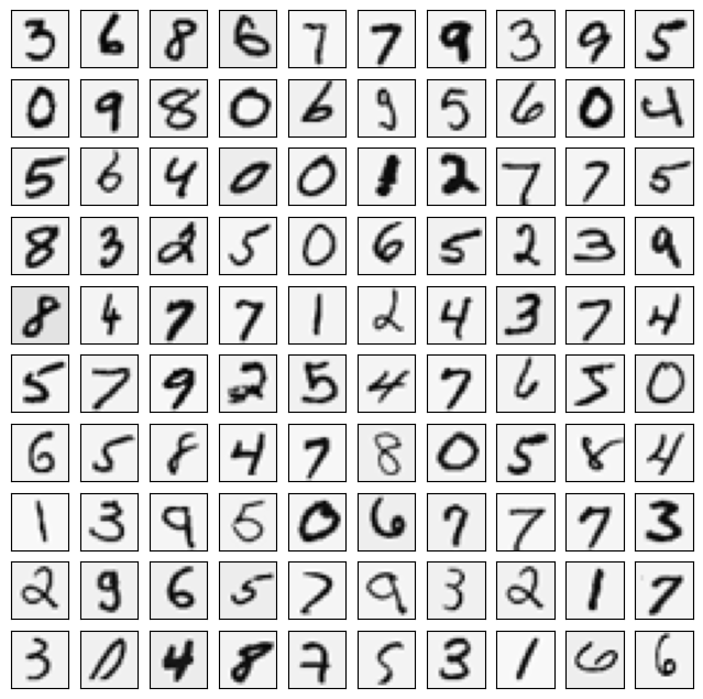
def plot_100_image(X):
    
    sample_index=np.random.choice(len(X),100)
    images=X[sample_index,:]
    print(images.shape)
    
    fig,ax=plt.subplots(ncols=10,nrows=10,figsize=(8,8,),sharex=True,sharey=True)
 
    for r in range(10):
        for c in range(10):
            ax[r,c].imshow(images[10*r+c].reshape(20,20).T,cmap='gray_r')
    
    plt.xticks([])
    plt.yticks([])
    plt.show

1 2	plot_100_image(raw_X) (100, 400)

png

损失函数与梯度下降

1 2	def sigmoid(z): return 1/(1+np.exp(-z))

def costFunction(theta,X,y,lamda):
    
    first=y*np.log(sigmoid(X@theta))
    second=(1-y)*np.log(1-sigmoid(X@theta))
    
    reg=theta[1:]@theta[1:]*(lamda/(2*len(X)))
    return -np.sum(first+second)/len(X)+reg

def gradient_reg(theta,X,y,lamda):
    reg=theta[1:]*(lamda/len(X))
    reg=np.insert(reg,0,values=0,axis=0)
    
    first=(X.T@(sigmoid(X@theta)-y))/len(X)
    
    return first+reg

X=np.insert(raw_X,0,values=1,axis=1)
X.shape
(5000, 401)
y=raw_y.flatten()
y.shape
(5000,)

模型生成

from scipy.optimize import minimize

def one_vs_all(X,y,lamda,K):
    
    n=X.shape[1]
    
    theta_all=np.zeros((K,n))
    
    for i in range(1,K+1):
        theta_i=np.zeros(n,)
        
        res=minimize(fun=costFunction,x0=theta_i,args=(X,y==i,lamda),method='TNC',jac=gradient_reg)
        theta_all[i-1,:]=res.x
        
    return theta_all

lamda=1
K=10
theta_final=one_vs_all(X,y,lamda,K)
theta_final

array([[-2.38187334e+00,  0.00000000e+00,  0.00000000e+00, ...,
         1.30433279e-03, -7.29580949e-10,  0.00000000e+00],
       [-3.18303389e+00,  0.00000000e+00,  0.00000000e+00, ...,
         4.46340729e-03, -5.08870029e-04,  0.00000000e+00],
       [-4.79638233e+00,  0.00000000e+00,  0.00000000e+00, ...,
        -2.87468695e-05, -2.47395863e-07,  0.00000000e+00],
       ...,
       [-7.98700752e+00,  0.00000000e+00,  0.00000000e+00, ...,
        -8.94576566e-05,  7.21256372e-06,  0.00000000e+00],
       [-4.57358931e+00,  0.00000000e+00,  0.00000000e+00, ...,
        -1.33390955e-03,  9.96868542e-05,  0.00000000e+00],
       [-5.40542751e+00,  0.00000000e+00,  0.00000000e+00, ...,
        -1.16613537e-04,  7.88124085e-06,  0.00000000e+00]])

预测结果准确率

将预测结果1的位置与图片实际的数字序号（1）的位置进行比对，相同则记1，不同则记0。将结果累加并除以测试用数据个数，即可得到准确率。

def predict(X,theta_final):
    
    h=sigmoid(X@theta_final.T)
    
    h_argmax=np.argmax(h,axis=1)
    
    return h_argmax+1

y_pred=predict(X,theta_final)
acc=np.mean(y_pred==y)
acc
0.9446

实际图片与预测结果的比对

该模型用训练集进行检测准确率为0.9446，从下面随机选取的10个样本可以看见，该模型错把一个5认成了9。

def plot_an_image_test(X,X_2):
    
    pick_test=np.random.randint(5000)
    
    image=X[pick_test,:]
    
    fig,ax=plt.subplots(figsize=(1,1))
    ax.imshow(image.reshape(20,20).T,cmap='gray_r')
    
    plt.xticks([])
    plt.yticks([])

    
    test_result=sigmoid(X_2[pick_test,:]@theta_final.T)
    test_answer=np.argmax(test_result)
    
    print(f"数字判断为",(0 if test_answer+1==10 else test_answer+1),f"实际为",(0 if raw_y[pick_test,0]==10 else raw_y[pick_test,0]))

for i in range(10): 
    plot_an_image_test(raw_X,X)

数字判断为 1 实际为 1
数字判断为 2 实际为 2
数字判断为 3 实际为 3
数字判断为 9 实际为 9
数字判断为 8 实际为 8
数字判断为 9 实际为 5
数字判断为 4 实际为 4
数字判断为 3 实际为 3
数字判断为 2 实际为 2
数字判断为 7 实际为 7